In this guide, you’ll find a useful cheat sheet that documents some of the more commonly used elements of SQL, and even a few of the less common. Hopefully, it will help developers – both beginner and experienced level – become more proficient in their understanding of the SQL language.
Use this as a quick reference during development, a learning aid, or even print it out and bind it if you’d prefer (whatever works!).
But before we get to the cheat sheet itself, for developers who may not be familiar with SQL, let’s start with…
PDF Version of SQL Cheat Sheet
SQL Cheat Sheet (Download PDF)
What is SQL
SQL stands for Structured Query Language. It’s the language of choice on today’s web for storing, manipulating and retrieving data within relational databases. Most, if not all of the websites you visit will use it in some way, including this one.
Here’s what a basic relational database looks like. This example in particular stores e-commerce information, specifically the products on sale, the users who buy them, and records of these orders which link these 2 entities.

Using SQL, you are able to interact with the database by writing queries, which when executed, return any results which meet its criteria.
Here’s an example query:-
SELECT * FROM users;
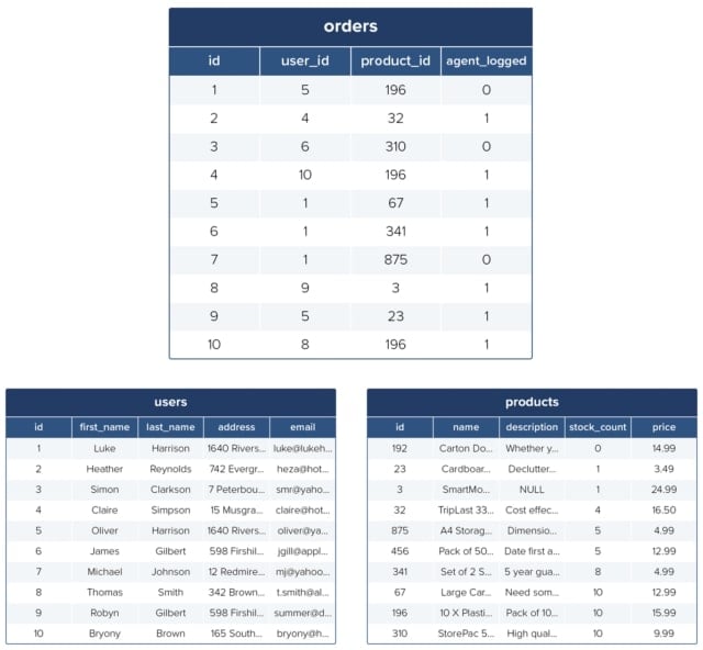
Using this SELECT statement, the query selects all data from all columns in the user’s table. It would then return data like the below, which is typically called a results set:-

If we were to replace the asterisk wildcard character (*) with specific column names instead, only the data from these columns would be returned from the query.
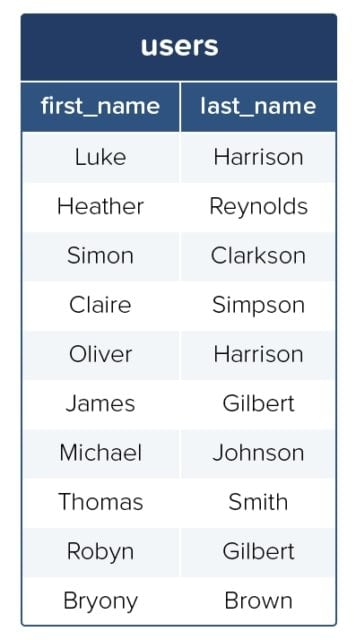
SELECT first_name, last_name FROM users;
We can add a bit of complexity to a standard SELECT statement by adding a WHERE clause, which allows you to filter what gets returned.
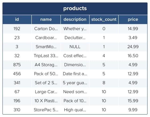
SELECT * FROM products WHERE stock_count <= 10 ORDER BY stock_count ASC;
This query would return all data from the products table with a stock_count value of less than 10 in its results set.
The use of the ORDER BY keyword means the results will be ordered using the stock_count column, lowest values to highest.
Using the INSERT INTO statement, we can add new data to a table. Here’s a basic example adding a new user to the users table:-
INSERT INTO users (first_name, last_name, address, email)
VALUES ('Tester', 'Jester', '123 Fake Street, Sheffield, United Kingdom', 'test@lukeharrison.dev');
Then if you were to rerun the query to return all data from the user’s table, the results set would look like this:

Of course, these examples demonstrate only a very small selection of what the SQL language is capable of.
SQL vs MySQL
You may have heard of MySQL before. It’s important that you don’t confuse this with SQL itself, as there’s a clear difference.
 SQL is the language. It outlines syntax that allows you to write queries that manage relational databases. Nothing more.
MySQL meanwhile is a database system that runs on a server. It implements the SQL language, allowing you to write queries using its syntax to manage MySQL databases.
In addition to MySQL, there are other systems that implement SQL. Some of the more popular ones include:
- PostgreSQL
- SQLite
- Oracle Database
- Microsoft SQL Server
Installing MySQL
Windows
The recommended way to install MySQL on Windows is by using the installer you can download from the MySQL website.

MacOS
On macOS, the recommended way to install MySQL is using native packages, which sounds a lot more complicated than it actually is. Essentially, it also involves just downloading an installer.

Alternatively, If you prefer to use package managers such as Homebrew, you can install MySQL like so:
brew install mysql
Whilst if you need to install the older MySQL version 5.7, which is still widely used today on the web, you can:
brew install mysql@5.7
Using MySQL
With MySQL now installed on your system, to get up and going as quickly as possible writing SQL queries, it’s recommended that you use an SQL management application to make managing your databases a much simpler, easier process.
There are lots of apps to choose from which largely do the same job, so it’s down to your own personal preference on which one to use:
- MySQL Workbench is developed by Oracle, the owner of MySQL.
- HeidiSQL (Recommended Windows) is a free, open-source app for Windows. For macOS and Linux users, Wine is first required as a prerequisite.
- phpMyAdmin is a very popular alternative that operates in the web browser.
- Sequel Pro (Recommended macOS) is a macOS’ only alternative and our favorite thanks to its clear and easy to use interface.
When you’re ready to start writing your own SQL queries, rather than spending time creating your own database, consider importing dummy data instead.
The MySQL website provides a number of dummy databases that you can download free of charge and then import into your SQL app.

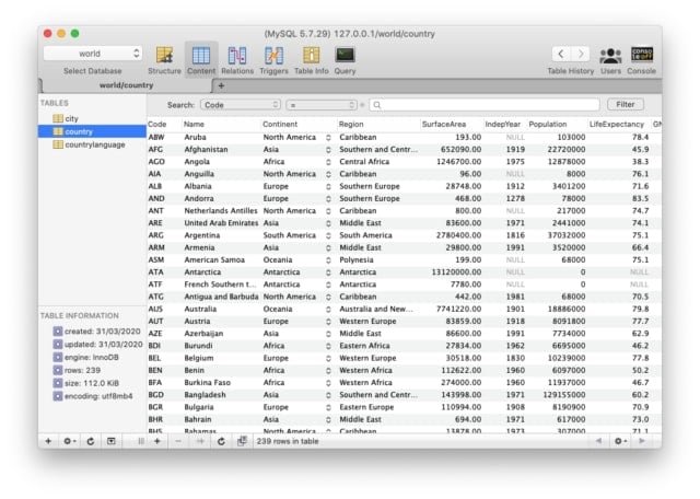
Our favorite of these is the world database, which provides some interesting data to practice writing SQL queries for. Here’s a screenshot of its country table within Sequel Pro.
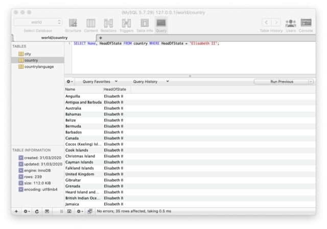
This example query returns all countries with Queen Elizabeth II as their head of state.
Whilst this one returns all European countries with a population of over 50million along with their capital city and its population.
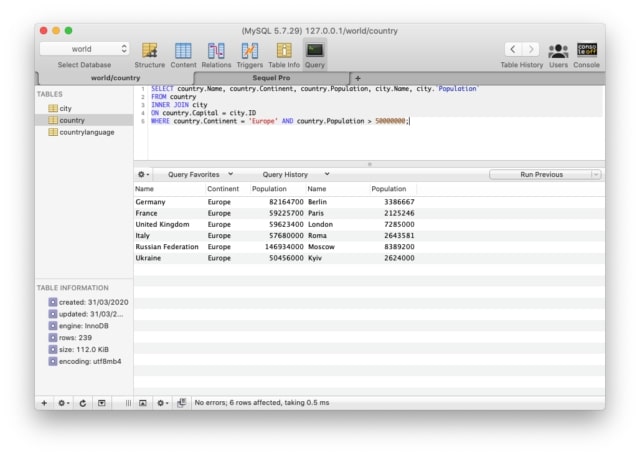
And this final one returns the average percentage of French speakers in countries where the total number of French speakers is higher than 10%.

Cheat Sheet
Keywords
A collection of keywords used in SQL statements, a description, and where appropriate an example. Some of the more advanced keywords have their own dedicated section later in the cheat sheet.
Where MySQL is mentioned next to an example, this means this example is only applicable to MySQL databases (as opposed to any other database system).
| SQL Keywords | |
|---|---|
| Keyword | Description |
| ADD | Adds a new column to an existing table.
Example: Adds a new column named ‘email_address’ to a table named ‘users’. ALTER TABLE users ADD email_address varchar(255); |
| ADD CONSTRAINT | It creates a new constraint on an existing table, which is used to specify rules for any data in the table.
Example: Adds a new PRIMARY KEY constraint named ‘user’ on columns ID and SURNAME. ALTER TABLE users ADD CONSTRAINT user PRIMARY KEY (ID, SURNAME); |
| ALTER TABLE | Adds, deletes or edits columns in a table. It can also be used to add and delete constraints in a table, as per the above.
Example: Adds a new boolean column called ‘approved’ to a table named ‘deals’. ALTER TABLE deals ADD approved boolean; Example 2: Deletes the ‘approved’ column from the ‘deals’ table ALTER TABLE deals DROP COLUMN approved; |
| ALTER COLUMN | Changes the data type of a table’s column.
Example: In the ‘users’ table, make the column ‘incept_date’ into a ‘datetime’ type. ALTER TABLE users ALTER COLUMN incept_date datetime; |
| ALL | Returns true if all of the subquery values meet the passed condition.
Example: Returns the users with a higher number of tasks than the user with the highest number of tasks in the HR department (id 2) SELECT first_name, surname, tasks_no FROM users WHERE tasks_no > ALL (SELECT tasks FROM user WHERE department_id = 2); |
| AND | Used to join separate conditions within a WHERE clause.
Example: Returns events located in London, United Kingdom SELECT * FROM events WHERE host_country='United Kingdom' AND host_city='London'; |
| ANY | Returns true if any of the subquery values meet the given condition.
Example: Returns products from the products table which have received orders – stored in the orders table – with a quantity of more than 5. SELECT name FROM products WHERE productId = ANY (SELECT productId FROM orders WHERE quantity > 5); |
| AS | Renames a table or column with an alias value which only exists for the duration of the query.
Example: Aliases north_east_user_subscriptions column SELECT north_east_user_subscriptions AS ne_subs FROM users WHERE ne_subs > 5; |
| ASC | Used with ORDER BY to return the data in ascending order.
Example: Apples, Bananas, Peaches, Raddish |
| BETWEEN | Selects values within the given range.
Example 1: Selects stock with a quantity between 100 and 150. SELECT * FROM stock WHERE quantity BETWEEN 100 AND 150; Example 2: Selects stock with a quantity NOT between 100 and 150. Alternatively, using the NOT keyword here reverses the logic and selects values outside the given range. SELECT * FROM stock WHERE quantity NOT BETWEEN 100 AND 150; |
| CASE | Change query output depending on conditions.
Example: Returns users and their subscriptions, along with a new column called activity_levels that makes a judgement based on the number of subscriptions. SELECT first_name, surname, subscriptions CASE WHEN subscriptions > 10 THEN 'Very active' WHEN Quantity BETWEEN 3 AND 10 THEN 'Active' ELSE 'Inactive' END AS activity_levels FROM users; |
| CHECK | Adds a constraint that limits the value which can be added to a column.
Example 1 (MySQL): Makes sure any users added to the users table are 18 or over. CREATE TABLE users ( first_name varchar(255), age int, CHECK (age>=18) ); Example 2 (MySQL): Adds a check after the table has already been created. ALTER TABLE users ADD CHECK (age>=18); |
| CREATE DATABASE | Creates a new database.
Example: Creates a new database named ‘websitesetup’. CREATE DATABASE websitesetup; |
| CREATE TABLE | Creates a new table .
Example: Creates a new table called ‘users’ in the ‘websitesetup’ database. CREATE TABLE users ( id int, first_name varchar(255), surname varchar(255), address varchar(255), contact_number int ); |
| DEFAULT | Sets a default value for a column;
Example 1 (MySQL): Creates a new table called Products which has a name column with a default value of ‘Placeholder Name’ and an available_from column with a default value of today’s date. CREATE TABLE products ( id int, name varchar(255) DEFAULT 'Placeholder Name', available_from date DEFAULT GETDATE() ); Example 2 (MySQL): The same as above, but editing an existing table. ALTER TABLE products ALTER name SET DEFAULT 'Placeholder Name', ALTER available_from SET DEFAULT GETDATE(); |
| DELETE | Delete data from a table.
Example: Removes a user with a user_id of 674. DELETE FROM users WHERE user_id = 674; |
| DESC | Used with ORDER BY to return the data in descending order.
Example: Raddish, Peaches, Bananas, Apples |
| DROP COLUMN | Deletes a column from a table.
Example: Removes the first_name column from the users table. ALTER TABLE users DROP COLUMN first_name |
| DROP DATABASE | Deletes the entire database.
Example: Deletes a database named ‘websitesetup’. DROP DATABASE websitesetup; |
| DROP DEFAULT | Removes a default value for a column.
Example (MySQL): Removes the default value from the ‘name’ column in the ‘products’ table. ALTER TABLE products ALTER COLUMN name DROP DEFAULT; |
| DROP TABLE | Deletes a table from a database.
Example: Removes the users table. DROP TABLE users; |
| EXISTS | Checks for the existence of any record within the subquery, returning true if one or more records are returned.
Example: Lists any dealerships with a deal finance percentage less than 10. SELECT dealership_name FROM dealerships WHERE EXISTS (SELECT deal_name FROM deals WHERE dealership_id = deals.dealership_id AND finance_percentage < 10); |
| FROM | Specifies which table to select or delete data from.
Example: Selects data from the users table. SELECT area_manager FROM area_managers WHERE EXISTS (SELECT ProductName FROM Products WHERE area_manager_id = deals.area_manager_id AND Price < 20); |
| IN | Used alongside a WHERE clause as a shorthand for multiple OR conditions.
So instead of:- SELECT * FROM users WHERE country = 'USA' OR country = 'United Kingdom' OR country = 'Russia' OR country = 'Australia'; You can use:- SELECT * FROM users
WHERE country IN ('USA', 'United Kingdom', 'Russia', 'Australia');
|
| INSERT INTO | Add new rows to a table.
Example: Adds a new vehicle. INSERT INTO cars (make, model, mileage, year)
VALUES ('Audi', 'A3', 30000, 2016);
|
| IS NULL | Tests for empty (NULL) values.
Example: Returns users that haven’t given a contact number. SELECT * FROM users WHERE contact_number IS NULL; |
| IS NOT NULL | The reverse of NULL. Tests for values that aren’t empty / NULL. |
| LIKE | Returns true if the operand value matches a pattern.
Example: Returns true if the user’s first_name ends with ‘son’. SELECT * FROM users WHERE first_name LIKE '%son'; |
| NOT | Returns true if a record DOESN’T meet the condition.
Example: Returns true if the user’s first_name doesn’t end with ‘son’. SELECT * FROM users WHERE first_name NOT LIKE '%son'; |
| OR | Used alongside WHERE to include data when either condition is true.
Example: Returns users that live in either Sheffield or Manchester. SELECT * FROM users WHERE city = 'Sheffield' OR 'Manchester'; |
| ORDER BY | Used to sort the result data in ascending (default) or descending order through the use of ASC or DESC keywords.
Example: Returns countries in alphabetical order. SELECT * FROM countries ORDER BY name; |
| ROWNUM | Returns results where the row number meets the passed condition.
Example: Returns the top 10 countries from the countries table. SELECT * FROM countries WHERE ROWNUM <= 10; |
| SELECT | Used to select data from a database, which is then returned in a results set.
Example 1: Selects all columns from all users. SELECT * FROM users; Example 2: Selects the first_name and surname columns from all users.xx SELECT first_name, surname FROM users; |
| SELECT DISTINCT | Sames as SELECT, except duplicate values are excluded.
Example: Creates a backup table using data from the users table. SELECT * INTO usersBackup2020 FROM users; |
| SELECT INTO | Copies data from one table and inserts it into another.
Example: Returns all countries from the users table, removing any duplicate values (which would be highly likely) SELECT DISTINCT country from users; |
| SELECT TOP | Allows you to return a set number of records to return from a table.
Example: Returns the top 3 cars from the cars table. SELECT TOP 3 * FROM cars; |
| SET | Used alongside UPDATE to update existing data in a table.
Example: Updates the value and quantity values for an order with an id of 642 in the orders table. UPDATE orders SET value = 19.49, quantity = 2 WHERE id = 642; |
| SOME | Identical to ANY. |
| TOP | Used alongside SELECT to return a set number of records from a table.
Example: Returns the top 5 users from the users table. SELECT TOP 5 * FROM users; |
| TRUNCATE TABLE | Similar to DROP, but instead of deleting the table and its data, this deletes only the data.
Example: Empties the sessions table, but leaves the table itself intact. TRUNCATE TABLE sessions; |
| UNION | Combines the results from 2 or more SELECT statements and returns only distinct values.
Example: Returns the cities from the events and subscribers tables. SELECT city FROM events UNION SELECT city from subscribers; |
| UNION ALL | The same as UNION, but includes duplicate values. |
| UNIQUE | This constraint ensures all values in a column are unique.
Example 1 (MySQL): Adds a unique constraint to the id column when creating a new users table. CREATE TABLE users ( id int NOT NULL, name varchar(255) NOT NULL, UNIQUE (id) ); Example 2 (MySQL): Alters an existing column to add a UNIQUE constraint. ALTER TABLE users ADD UNIQUE (id);
|
| UPDATE | Updates existing data in a table.
Example: Updates the mileage and serviceDue values for a vehicle with an id of 45 in the cars table. UPDATE cars SET mileage = 23500, serviceDue = 0 WHERE id = 45; |
| VALUES | Used alongside the INSERT INTO keyword to add new values to a table.
Example: Adds a new car to the cars table. INSERT INTO cars (name, model, year)
VALUES ('Ford', 'Fiesta', 2010);
|
| WHERE | Filters results to only include data which meets the given condition.
Example: Returns orders with a quantity of more than 1 item. SELECT * FROM orders WHERE quantity > 1; |
Comments
Comments allow you to explain sections of your SQL statements, or to comment out code and prevent its execution.
In SQL, there are 2 types of comments, single line and multiline.
Single Line Comments
Single line comments start with –. Any text after these 2 characters to the end of the line will be ignored.
-- My Select query
SELECT * FROM users;
Multiline Comments
Multiline comments start with /* and end with */. They stretch across multiple lines until the closing characters have been found.
/*
This is my select query.
It grabs all rows of data from the users table
*/
SELECT * FROM users;

/*
This is another select query, which I don't want to execute yet

SELECT * FROM tasks;
*/
MySQL Data Types
When creating a new table or editing an existing one, you must specify the type of data that each column accepts.
In the below example, data passed to the id column must be an int, whilst the first_name column has a VARCHAR data type with a maximum of 255 characters.
CREATE TABLE users (
    id int,
    first_name varchar(255)
);
String Data Types
| String Data Types | ||
|---|---|---|
| Data Type | Description | |
| CHAR(size) | Fixed length string which can contain letters, numbers and special characters. The size parameter sets the maximum string length, from 0 – 255 with a default of 1. | |
| VARCHAR(size) | Variable length string similar to CHAR(), but with a maximum string length range from 0 to 65535. | |
| BINARY(size) | Similar to CHAR() but stores binary byte strings. | |
| VARBINARY(size) | Similar to VARCHAR() but for binary byte strings. | |
| TINYBLOB | Holds Binary Large Objects (BLOBs) with a max length of 255 bytes. | |
| TINYTEXT | Holds a string with a maximum length of 255 characters. Use VARCHAR() instead, as it’s fetched much faster. | |
| TEXT(size) | Holds a string with a maximum length of 65535 bytes. Again, better to use VARCHAR(). | |
| BLOB(size) | Holds Binary Large Objects (BLOBs) with a max length of 65535 bytes. | |
| MEDIUMTEXT | Holds a string with a maximum length of 16,777,215 characters. | |
| MEDIUMBLOB | Holds Binary Large Objects (BLOBs) with a max length of 16,777,215 bytes. | |
| LONGTEXT | Holds a string with a maximum length of 4,294,967,295 characters. | |
| LONGBLOB | Holds Binary Large Objects (BLOBs) with a max length of 4,294,967,295 bytes. | |
| ENUM(a, b, c, etc…) | A string object that only has one value, which is chosen from a list of values which you define, up to a maximum of 65535 values. If a value is added which isn’t on this list, it’s replaced with a blank value instead. Think of ENUM being similar to HTML radio boxes in this regard.
|
|
| SET(a, b, c, etc…) | A string object that can have 0 or more values, which is chosen from a list of values which you define, up to a maximum of 64 values. Think of SET being similar to HTML checkboxes in this regard. | |
Numeric Data Types
| String Data Types | |
|---|---|
| Data Type | Description |
| BIT(size) | A bit-value type with a default of 1. The allowed number of bits in a value is set via the size parameter, which can hold values from 1 to 64. |
| TINYINT(size) | A very small integer with a signed range of -128 to 127, and an unsigned range of 0 to 255. Here, the size parameter specifies the maximum allowed display width, which is 255. |
| BOOL | Essentially a quick way of setting the column to TINYINT with a size of 1. 0 is considered false, whilst 1 is considered true. |
| BOOLEAN | Same as BOOL. |
| SMALLINT(size) | A small integer with a signed range of -32768 to 32767, and an unsigned range from 0 to 65535. Here, the size parameter specifies the maximum allowed display width, which is 255. |
| MEDIUMINT(size) | A medium integer with a signed range of -8388608 to 8388607, and an unsigned range from 0 to 16777215. Here, the size parameter specifies the maximum allowed display width, which is 255. |
| INT(size) | A medium integer with a signed range of -2147483648 to 2147483647, and an unsigned range from 0 to 4294967295. Here, the size parameter specifies the maximum allowed display width, which is 255. |
| INTEGER(size) | Same as INT. |
| BIGINT(size) | A medium integer with a signed range of -9223372036854775808 to 9223372036854775807, and an unsigned range from 0 to 18446744073709551615. Here, the size parameter specifies the maximum allowed display width, which is 255. |
| FLOAT(p) | A floating point number value. If the precision (p) parameter is between 0 to 24, then the data type is set to FLOAT(), whilst if its from 25 to 53, the data type is set to DOUBLE(). This behaviour is to make the storage of values more efficient. |
| DOUBLE(size, d) | A floating point number value where the total digits are set by the size parameter, and the number of digits after the decimal point is set by the d parameter. |
| DECIMAL(size, d) | An exact fixed point number where the total number of digits is set by the size parameters, and the total number of digits after the decimal point is set by the d parameter.
For size, the maximum number is 65 and the default is 10, whilst for d, the maximum number is 30 and the default is 10. |
| DEC(size, d) | Same as DECIMAL. |
Date / Time Data Types
| Date / Time Data Types | |
|---|---|
| Data Type | Description |
| DATE | A simple date in YYYY-MM–DD format, with a supported range from ‘1000-01-01’ to ‘9999-12-31’. |
| DATETIME(fsp) | A date time in YYYY-MM-DD hh:mm:ss format, with a supported range from ‘1000-01-01 00:00:00’ to ‘9999-12-31 23:59:59’.
By adding DEFAULT and ON UPDATE to the column definition, it automatically sets to the current date/time. |
| TIMESTAMP(fsp) | A Unix Timestamp, which is a value relative to the number of seconds since the Unix epoch (‘1970-01-01 00:00:00’ UTC). This has a supported range from ‘1970-01-01 00:00:01’ UTC to ‘2038-01-09 03:14:07’ UTC.
By adding DEFAULT CURRENT_TIMESTAMP and ON UPDATE CURRENT TIMESTAMP to the column definition, it automatically sets to current date/time. |
| TIME(fsp) | A time in hh:mm:ss format, with a supported range from ‘-838:59:59’ to ‘838:59:59’. |
| YEAR | A year, with a supported range of ‘1901’ to ‘2155’. |
Operators
Arithmetic Operators
| Arithmetic Operators | |
|---|---|
| Operator | Description |
| + | Add |
| – | Subtract |
| * | Multiply |
| / | Divide |
| % | Modulo |
Bitwise Operator
| Bitwise Operators | |
|---|---|
| Operator | Description |
| & | Bitwise AND |
| | | Bitwise OR |
| ^ | Bitwise exclusive OR |
Comparison Operators
| Comparison Operators | |
|---|---|
| Operator | Description |
| = | Equal to |
| > | Greater than |
| < | Less than |
| >= | Greater than or equal to |
| <= | Less than or equal to |
| <> | Not equal to |
Compound Operators
| Compound Operators | |
|---|---|
| Operator | Description |
| += | Add equals |
| -= | Subtract equals |
| *= | Multiply equals |
| /= | Divide equals |
| %= | Modulo equals |
| &= | Bitwise AND equals |
| ^-= | Bitwise exclusive equals |
| |*= | Bitwise OR equals |
Functions
String Functions
| String Functions | |
|---|---|
| Name | Description |
| ASCII | Returns the equivalent ASCII value for a specific character. |
| CHAR_LENGTH | Returns the character length of a string. |
| CHARACTER_LENGTH | Same as CHAR_LENGTH. |
| CONCAT | Adds expressions together, with a minimum of 2. |
| CONCAT_WS | Adds expressions together, but with a separator between each value. |
| FIELD | Returns an index value relative to the position of a value within a list of values. |
| FIND IN SET | Returns the position of a string in a list of strings. |
| FORMAT | When passed a number, returns that number formatted to include commas (eg 3,400,000). |
| INSERT | Allows you to insert one string into another at a certain point, for a certain number of characters. |
| INSTR | Returns the position of the first time one string appears within another. |
| LCASE | Convert a string to lowercase. |
| LEFT | Starting from the left, extract the given number of characters from a string and return them as another. |
| LENGTH | Returns the length of a string, but in bytes. |
| LOCATE | Returns the first occurrence of one string within another, |
| LOWER | Same as LCASE. |
| LPAD | Left pads one string with another, to a specific length. |
| LTRIM | Remove any leading spaces from the given string. |
| MID | Extracts one string from another, starting from any position. |
| POSITION | Returns the position of the first time one substring appears within another. |
| REPEAT | Allows you to repeat a string |
| REPLACE | Allows you to replace any instances of a substring within a string, with a new substring. |
| REVERSE | Reverses the string. |
| RIGHT | Starting from the right, extract the given number of characters from a string and return them as another. |
| RPAD | Right pads one string with another, to a specific length. |
| RTRIM | Removes any trailing spaces from the given string. |
| SPACE | Returns a string full of spaces equal to the amount you pass it. |
| STRCMP | Compares 2 strings for differences |
| SUBSTR | Extracts one substring from another, starting from any position. |
| SUBSTRING | Same as SUBSTR |
| SUBSTRING_INDEX | Returns a substring from a string before the passed substring is found the number of times equals to the passed number. |
| TRIM | Removes trailing and leading spaces from the given string. Same as if you were to run LTRIM and RTRIM together. |
| UCASE | Convert a string to uppercase. |
| UPPER | Same as UCASE. |
Numeric Functions
| Numeric Functions | |
|---|---|
| Name | Description |
| ABS | Returns the absolute value of the given number. |
| ACOS | Returns the arc cosine of the given number. |
| ASIN | Returns the arc sine of the given number. |
| ATAN | Returns the arc tangent of one or 2 given numbers. |
| ATAN2 | Return the arc tangent of 2 given numbers. |
| AVG | Returns the average value of the given expression. |
| CEIL | Returns the closest whole number (integer) upwards from a given decimal point number. |
| CEILING | Same as CEIL. |
| COS | Returns the cosine of a given number. |
| COT | Returns the cotangent of a given number. |
| COUNT | Returns the amount of records that are returned by a SELECT query. |
| DEGREES | Converts a radians value to degrees. |
| DIV | Allows you to divide integers. |
| EXP | Returns e to the power of the given number. |
| FLOOR | Returns the closest whole number (integer) downwards from a given decimal point number. |
| GREATEST | Returns the highest value in a list of arguments. |
| LEAST | Returns the smallest value in a list of arguments. |
| LN | Returns the natural logarithm of the given number |
| LOG | Returns the natural logarithm of the given number, or the logarithm of the given number to the given base |
| LOG10 | Does the same as LOG, but to base 10. |
| LOG2 | Does the same as LOG, but to base 2. |
| MAX | Returns the highest value from a set of values. |
| MIN | Returns the lowest value from a set of values. |
| MOD | Returns the remainder of the given number divided by the other given number. |
| PI | Returns PI. |
| POW | Returns the value of the given number raised to the power of the other given number. |
| POWER | Same as POW. |
| RADIANS | Converts a degrees value to radians. |
| RAND | Returns a random number. |
| ROUND | Round the given number to the given amount of decimal places. |
| SIGN | Returns the sign of the given number. |
| SIN | Returns the sine of the given number. |
| SQRT | Returns the square root of the given number. |
| SUM | Returns the value of the given set of values combined. |
| TAN | Returns the tangent of the given number. |
| TRUNCATE | Returns a number truncated to the given number of decimal places. |
Date Functions
| Date Functions | |
|---|---|
| Name | Description |
| ADDDATE | Add a date interval (eg: 10 DAY) to a date (eg: 20/01/20) and return the result (eg: 20/01/30). |
| ADDTIME | Add a time interval (eg: 02:00) to a time or datetime (05:00) and return the result (07:00). |
| CURDATE | Get the current date. |
| CURRENT_DATE | Same as CURDATE. |
| CURRENT_TIME | Get the current time. |
| CURRENT_TIMESTAMP | Get the current date and time. |
| CURTIME | Same as CURRENT_TIME. |
| DATE | Extracts the date from a datetime expression. |
| DATEDIFF | Returns the number of days between the 2 given dates. |
| DATE_ADD | Same as ADDDATE. |
| DATE_FORMAT | Formats the date to the given pattern. |
| DATE_SUB | Subtract a date interval (eg: 10 DAY) to a date (eg: 20/01/20) and return the result (eg: 20/01/10). |
| DAY | Returns the day for the given date. |
| DAYNAME | Returns the weekday name for the given date. |
| DAYOFWEEK | Returns the index for the weekday for the given date. |
| DAYOFYEAR | Returns the day of the year for the given date. |
| EXTRACT | Extract from the date the given part (eg MONTH for 20/01/20 = 01). |
| FROM DAYS | Return the date from the given numeric date value. |
| HOUR | Return the hour from the given date. |
| LAST DAY | Get the last day of the month for the given date. |
| LOCALTIME | Gets the current local date and time. |
| LOCALTIMESTAMP | Same as LOCALTIME. |
| MAKEDATE | Creates a date and returns it, based on the given year and number of days values. |
| MAKETIME | Creates a time and returns it, based on the given hour, minute and second values. |
| MICROSECOND | Returns the microsecond of a given time or datetime. |
| MINUTE | Returns the minute of the given time or datetime. |
| MONTH | Returns the month of the given date. |
| MONTHNAME | Returns the name of the month of the given date. |
| NOW | Same as LOCALTIME. |
| PERIOD_ADD | Adds the given number of months to the given period. |
| PERIOD_DIFF | Returns the difference between 2 given periods. |
| QUARTER | Returns the year quarter for the given date. |
| SECOND | Returns the second of a given time or datetime. |
| SEC_TO_TIME | Returns a time based on the given seconds. |
| STR_TO_DATE | Creates a date and returns it based on the given string and format. |
| SUBDATE | Same as DATE_SUB. |
| SUBTIME | Subtracts a time interval (eg: 02:00) to a time or datetime (05:00) and return the result (03:00). |
| SYSDATE | Same as LOCALTIME. |
| TIME | Returns the time from a given time or datetime. |
| TIME_FORMAT | Returns the given time in the given format. |
| TIME_TO_SEC | Converts and returns a time into seconds. |
| TIMEDIFF | Returns the difference between 2 given time/datetime expressions. |
| TIMESTAMP | Returns the datetime value of the given date or datetime. |
| TO_DAYS | Returns the total number of days that have passed from ‘00-00-0000’ to the given date. |
| WEEK | Returns the week number for the given date. |
| WEEKDAY | Returns the weekday number for the given date. |
| WEEKOFYEAR | Returns the week number for the given date. |
| YEAR | Returns the year from the given date. |
| YEARWEEK | Returns the year and week number for the given date. |
Misc Functions
| Misc Functions | |
|---|---|
| Name | Description |
| BIN | Returns the given number in binary. |
| BINARY | Returns the given value as a binary string. |
| CAST | Convert one type into another. |
| COALESCE | From a list of values, return the first non-null value. |
| CONNECTION_ID | For the current connection, return the unique connection ID. |
| CONV | Convert the given number from one numeric base system into another. |
| CONVERT | Convert the given value into the given datatype or character set. |
| CURRENT_USER | Return the user and hostname which was used to authenticate with the server. |
| DATABASE | Get the name of the current database. |
| GROUP BY | Used alongside aggregate functions (COUNT, MAX, MIN, SUM, AVG) to group the results.
Example: Lists the number of users with active orders. SELECT COUNT(user_id), active_orders FROM users GROUP BY active_orders; |
| HAVING | It’s used in the place of WHERE with aggregate functions.
Example: Lists the number of users with active orders, but only include users with more than 3 active orders. SELECT COUNT(user_id), active_orders FROM users GROUP BY active_orders HAVING COUNT(user_id) > 3; |
| IF | If the condition is true return a value, otherwise return another value. |
| IFNULL | If the given expression equates to null, return the given value. |
| ISNULL | If the expression is null, return 1, otherwise return 0. |
| LAST_INSERT_ID | For the last row which was added or updated in a table, return the auto increment ID. |
| NULLIF | Compares the 2 given expressions. If they are equal, NULL is returned, otherwise the first expression is returned. |
| SESSION_USER | Return the current user and hostnames. |
| SYSTEM_USER | Same as SESSION_USER. |
| USER | Same as SESSION_USER. |
| VERSION | Returns the current version of the MySQL powering the database. |
Wildcard Characters
In SQL, Wildcards are special characters used with the LIKE and NOT LIKE keywords which allow us to search data with sophisticated patterns much more efficiently
| Wildcards | |
|---|---|
| Name | Description |
| % | Equates to zero or more characters.
Example 1: Find all users with surnames ending in ‘son’. SELECT * FROM users WHERE surname LIKE '%son'; Example 2: Find all users living in cities containing the pattern ‘che’ SELECT * FROM users WHERE city LIKE '%che%'; |
| _ | Equates to any single character.
Example: Find all users living in cities beginning with any 3 characters, followed by ‘chester’. SELECT * FROM users WHERE city LIKE '___chester'; |
| [charlist] | Equates to any single character in the list.
Example 1: Find all users with first names beginning with J, H or M. SELECT * FROM users WHERE first_name LIKE '[jhm]%'; Example 2: Find all users with first names beginning letters between A – L. SELECT * FROM users WHERE first_name LIKE '[a-l]%'; Example 3: Find all users with first names not ending with letters between n – s. SELECT * FROM users WHERE first_name LIKE '%[!n-s]'; |
Keys
In relational databases, there is a concept of primary and foreign keys. In SQL tables, these are included as constraints, where a table can have a primary key, a foreign key, or both.
Primary Key
A primary key allows each record in a table to be uniquely identified. There can only be one primary key per table, and you can assign this constraint to any single or combination of columns. However, this means each value within this column(s) must be unique.
Typically in a table, the primary key is an ID column, and is usually paired with the AUTO_INCREMENT keyword. This means the value increases automatically as new records are created.
Example 1 (MySQL)
Create a new table and set the primary key to the ID column.
CREATE TABLE users (
    id int NOT NULL AUTO_INCREMENT,
    first_name varchar(255),
    last_name varchar(255) NOT NULL,
    address varchar(255),
    email varchar(255),
    PRIMARY KEY (id)
);
Example 2 (MySQL)
Alter an existing table and set the primary key to the first_name column.
ALTER TABLE users
ADD PRIMARY KEY (first_name);
Foreign Key
A foreign key can be applied to one column or many and is used to link 2 tables together in a relational database.
As seen in the diagram below, the table containing the foreign key is called the child key, whilst the table which contains the referenced key, or candidate key, is called the parent table.
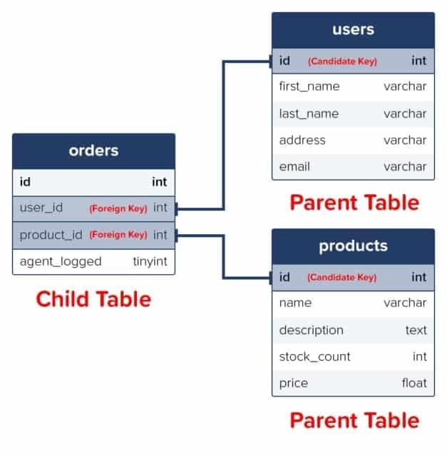
This essentially means that the column data is shared between 2 tables, as a foreign key also prevents invalid data from being inserted which isn’t also present in the parent table.
Example 1 (MySQL)
Create a new table and turn any columns that reference IDs in other tables into foreign keys.
CREATE TABLE orders (
    id int NOT NULL,
    user_id int,
    product_id int,
    PRIMARY KEY (id),
    FOREIGN KEY (user_id) REFERENCES users(id),
    FOREIGN KEY (product_id) REFERENCES products(id)
);
Example 2 (MySQL)
Alter an existing table and create a foreign key.
ALTER TABLE orders
ADD FOREIGN KEY (user_id) REFERENCES users(id);
Indexes
Indexes are attributes that can be assigned to columns that are frequently searched against to make data retrieval a quicker and more efficient process.
This doesn’t mean each column should be made into an index though, as it takes longer for a column with an index to be updated than a column without. This is because when indexed columns are updated, the index itself must also be updated.
| Indexes | |
|---|---|
| Name | Description |
| CREATE INDEX | Creates an index named ‘idx_test’ on the first_name and surname columns of the users table. In this instance, duplicate values are allowed.
CREATE INDEX idx_test ON users (first_name, surname); |
| CREATE UNIQUE INDEX | The same as the above, but no duplicate values.
CREATE UNIQUE INDEX idx_test ON users (first_name, surname); |
| DROP INDEX | Removes an index.
ALTER TABLE users DROP INDEX idx_test; |
Joins
In SQL, a JOIN clause is used to return a results set which combines data from multiple tables, based on a common column which is featured in both of them
There are a number of different joins available for you to use:-
- Inner Join (Default): Returns any records which have matching values in both tables.
- Left Join: Returns all of the records from the first table, along with any matching records from the second table.
- Right Join: Returns all of the records from the second table, along with any matching records from the first.
- Full Join: Returns all records from both tables when there is a match.
A common way of visualising how joins work is like this:

In the following example, an inner join will be used to create a new unifying view combining the orders table and then 3 different tables
We’ll replace the user_id and product_id with the first_name and surname columns of the user who placed the order, along with the name of the item which was purchased.
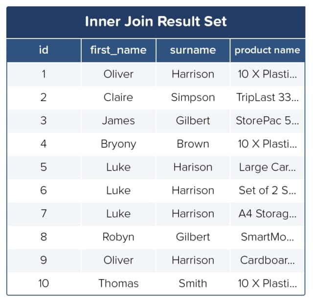
SELECT orders.id, users.first_name, users.surname, products.name as 'product name'
FROM orders
INNER JOIN users on orders.user_id = users.id
INNER JOIN products on orders.product_id = products.id;
Would return a results set which looks like:
View
A view is essentially a SQL results set that get stored in the database under a label, so you can return to it later, without having to rerun the query. These are especially useful when you have a costly SQL query which may be needed a number of times, so instead of running it over and over to generate the same results set, you can just do it once and save it as a view.
Creating Views
To create a view, you can do so like this:
CREATE VIEW priority_users AS
SELECT * FROM users
WHERE country = 'United Kingdom';
Then in future, if you need to access the stored result set, you can do so like this:
SELECT * FROM [priority_users];
Replacing Views
With the CREATE OR REPLACE command, a view can be updated.
CREATE OR REPLACE VIEW [priority_users] AS
SELECT * FROM users
WHERE country = 'United Kingdom' OR country='USA';
Deleting Views
To delete a view, simply use the DROP VIEW command.
DROP VIEW priority_users;
Conclusion
The majority of the websites on today’s web use relational databases in some way. This makes SQL a valuable language to know, as it allows you to create more complex, functional websites, and systems.
Make sure to bookmark this page, so in the future, if you’re working with SQL and can’t quite remember a specific operator, how to write a certain query, or are just confused about how joins work, then you’ll have a cheat sheet on hand which is ready, willing and able to help.
If you spot any errors in this cheat sheet, please contact us – info@websitesetup.org